
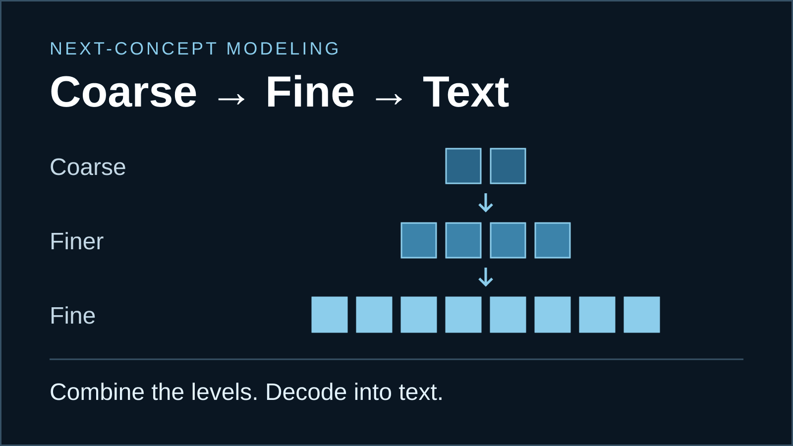
What if text generation started with the bigger picture?
Next-Concept Modeling changes the order in which a model produces its answer. For teams evaluating AI, it raises a useful question: how much of the wait comes from the way text is generated?
The October 9 preprint, Next-Concept Modeling: Fast, Parallel Coarse-to-Fine Text Generation, is by Hermann Kumbong, Ishan S. Khare and colleagues at Stanford and Together AI.
The authors’ research overview describes two sources of efficiency: fewer generation steps and less work in the early steps. Those early steps use shorter representations; later levels add detail.
How to read “concept.” The paper uses the term for information in coarse learned representations. It does not establish human-like understanding or a readable outline inside the model. Paper, §3.
Watch the generation order change
Choose a method, then play or step through the diagram. The animation illustrates dependencies, not measured running time. A box is a token position in next-token and masked-diffusion views, and a learned code in NCM.
Three ways to construct an answer
Same visual canvas. Different generation schedules.
NCM predicts one level at a time, with every code in that level generated together.
According to the released implementation, an NCM model pairs a frozen tokenizer with a generator. The tokenizer supplies the representation; the transformer learns to predict its levels. Its multiscale residual design lets later levels represent detail missing from the earlier reconstruction. “Coarse to fine” therefore describes the representation itself, rather than a prompt asking a model to write an outline.
Learn the representation
Train a multiscale tokenizer to encode text as discrete codes and reconstruct it.
Learn generation
Freeze the tokenizer. Train the transformer to predict levels from earlier reconstructions.
Think of the boxes as an explanation of where computation happens. They are not sentences being edited, and the animation is not a model running in your browser.
Strong speed results, with specific boundaries
Better generative perplexity than DUO.
Competitive generative perplexity versus the strongest diffusion baseline.
Comparable ROUGE-L versus AURORA-LM.
Most experiments use roughly 100-million-parameter generators; the LM1B scaling study reaches 725 million. Sudoku results favor NCM over the tested autoregressive and diffusion baselines. The authors identify fixed hierarchy schedules and occasional generation artifacts as limitations. Paper, §4.4 and Appendix I.
What this evidence leaves open. These results do not establish a universal speedup for a production assistant. A procurement decision still needs evidence about instruction following, factual accuracy, tool use, deployment constraints and the work your users actually perform.
How much of your workflow could actually get faster?
Editorial analysis: start with a latency breakdown. Document retrieval, external tools, network requests and human review can dominate a workflow. An improvement in generation affects only the portion spent generating.
A faster model changes one part of the clock.
Illustrative calculation: assume generation becomes 10× faster and everything else stays constant. This is a hypothetical scenario, not an NCM forecast.
If generation is half the wait, that hypothetical improvement makes the whole workflow about 1.82 times faster. This distinction matters when setting a pilot’s success criteria: measure the time to a usable, accepted answer.
For a bounded research pilot
Use a fixed document set and a written acceptance rubric. Compare completion time, factual errors, omitted details and reviewer effort. Keep hardware, batch size and output length in the results.
For a production decision
Require task-specific evidence at the intended scale. Include serving cost, operational ownership, monitoring and recovery. A benchmark ratio alone cannot answer those questions.
For an illustrative summarization pilot, ask reviewers to check names, dates, quantities and the main decision in every output. A summary that arrives sooner but needs more correction may offer little operational benefit. Record rejection rates alongside speed, and decide the quality threshold before comparing systems.
The official repository links checkpoints, evaluation datasets and task configurations for summarization, translation, Sudoku and unconditional generation. That gives technical teams a starting point for reproducible evaluation. Reproducing a benchmark and qualifying a business workflow remain separate milestones.
Our proposed next step is to add NCM to a research evaluation backlog if generation latency is a material bottleneck. Preserve your existing baseline, test one bounded task, and let accepted output quality determine whether further investment is justified.
Planning an evaluation? Use our guide to blind model evaluations to define a comparison around accepted output quality.
